Guyton-Klinger: Dynamic Withdrawal Strategy with Guardrails

January 25, 2026

Static inflation-indexed spending is simple, but it can be fragile in bad sequences and conservative in great markets. Guyton–Klinger adds explicit guardrails to adapt spending to portfolio conditions.

Continuing our theme of withdrawal strategy (you can read about our take on 4% withdrawal strategy here), let’s talk about a well-known dynamic withdrawal strategy - Guyton-Klinger.

Static withdrawals (the classic “4% rule”)

Each year, there are two key numbers:

• your portfolio balance at the start of the year (before you withdraw), and
• the dollar amount you plan to spend that year.

Under the classic inflation-indexed fixed-dollar rule, you:

• pick your first-year spending as a fixed percent of your starting portfolio (often 4%), then
• increase that same dollar amount each year with inflation—regardless of market performance.

Therefore, your spending amount, in real currency, is the same (i.e. same purchasing power). The benefit of this type of static spending is that it is predictable and it is easy. You can spend the same amount of money (in real terms) every year. However, there are two issues:

• This type of withdrawal policy is vulnerable to sequence-of-returns risks, that is, when the portfolio underperforms, the static spending will eat up the capital that is supposed to become the cushion in the future
• As illustrated in the back-testing in our previous post, the safe withdrawal rate may be higher than the 4% withdrawal rate, it means that the withdrawal rate may be conservative and hence the retiree is not able to “enjoy” the prosperity when the portfolio performs well.

In order to address these concerns, Guyton-Klinger (GK) proposes spending that adjusts based on portfolio performance. The four pillars are:

The advantage of dynamic withdrawal strategy like Guyton-Klinger is clear: by varying the spending (increasing in good years and decreasing in bad years), the retiree can expect the portfolio to last longer and hence a more robust retirement strategy than the static strategy.

What “Success” looks like in dynamic withdrawal strategy

In static withdrawal/spending rule, the definition of success is clear: the probability of not running out of money by the end of lifespan. However in dynamic withdrawal strategy, this is not a very satisfying scorecard – as in extreme scenarios, we may be forced to cut our spending to a level that is not sustainable. Therefore, a better approach, is to use spending outcome as the scorecard, for example:

1. Cut Frequency (number of years with a cut)
2. Time to first cut: how quickly the strategy demands austerity
3. Worst cut: the largest single-step reduction from one year to the next
4. Peak-to-trough spending decline: the largest drop from a local spending peak to the subsequent minimum
5. Number of years below a spending floor

Why we measure cut event? In dynamic withdrawal strategies, cuts matter because they are experienced as losses relative to a reference spending level. Losses carry disproportionate utility, hence they carry disproportionate utility weight: a $100 reduction in spending typically feels worse than a $100 increase feels good.

Exploring the Guyton-Klinger Strategy

To better understand how this strategy functions under various economic conditions, we've built an interactive calculator using shiller's market data^[1] and the original Guyton-Klinger paper^[2]:

Insights and Recommendations:

• Experiment with scenarios of lower expected returns by adjusting the "Return adjustment" under "Asset and Market" settings. Observe how the Guyton-Klinger strategy maintains portfolio resilience compared to static withdrawal method.
• Explore scenarios involving longer-than-expected lifespans by adjusting settings under "Horizon".

Visualizing Decisions over time

The following heatmaps compare Guyton-Klinger vs a plain CPI-indexed percentage withdrawal rule across start years 1960–1995:

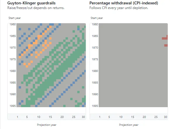
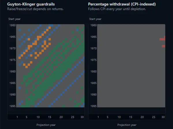
We can observe that while the fixed 4% rule typically ensures survival across most historical periods, there are notable exceptions when the market performed poorly. On the other hand, Guyton-Klinger strategy dynamically adapts the spending based on market performance, and was able to sustain more than 30 years for the "exception start years" for 4% rule. At other years, GK strategy increases the spending, allowing the retiree to enjoy the "prosperity" when their portfolio is doing well.

Adjusting parameters in the heatmap reveals that GK is especially valuable in scenarios with lower expected returns, highlighting its resilience in adverse market conditions.

Critiques and Considerations

While the Guyton-Klinger strategy offers significant benefits in terms of flexibility and portfolio resilience, it is not immune to some shortcomings:

• Risk of Overcorrection: Research indicates that GK's guardrails can be overly conservative, prompting spending cuts even in scenarios where they're not strictly necessary. For example, in extreme historical periods such as the Great Depression or the 1970s stagflation, the rules could have mandated real spending reduction exceeding 40%^[3]. Such significant cuts can be unpalatable to retirees.
• Behavioral Challenges: Frequent or deep spending cuts can be emotionally stressful, leading retirees to abandon the strategy prematurely or make less rational financial decisions during downturns.

Conclusion

The Guyton-Klinger withdrawal strategy offers retirees a structured yet dynamic approach that balances flexibility with security. By systematically adapting spending based on actual market performance, it addresses the vulnerabilities inherent in static strategies, enhancing long-term financial resilience and potentially increasing retiree satisfaction.

Ultimately, it's a tradeoff - the decision to adopt the Guyton-Klinger strategy depends on retirees' willingness to accept variability in spending to secure their financial future.

Sources

1. Shiller DataOnline dataRetrieved January 1, 2026. https://shillerdata.com/
2. FPA JournalDecision Rules and Maximum Initial Withdrawal RatesRetrieved January 18, 2026. https://www.financialplanningassociation.org/article/journal/MAR06-decision-rules-and-maximum-initial-withdrawal-rates
3. KitcesWhy Guyton-Klinger Guardrails Are Too Risky For Most Retirees (And How Risk-Based Guardrails Can Help)Retrieved January 18, 2026. https://www.kitces.com/blog/guyton-klinger-guardrails-retirement-income-rules-risk-based/